I’ve read quite a few presentations on Bayesian data analysis, but I always seem to fall into the crack between the first, one-step problem (the usual being how likely you are to have a disease), and more advanced problems that involve conjugate priors and quite a few other concepts. So, when I was recently reading Bayesian Data Analysis[1], I decided to tackle Exercise 13 from Chapter 2 using only Bayes rule updates and simulation. I think it’s been illuminating, so decided to write it up here, using my favorite tool R.

Exercise 13 involves annual airline accidents from 1976 to 1985, modeled as a Poisson distribution. The data is :

accidents <- c(24, 25, 31, 31, 22, 21, 26, 20, 16, 22)

A little playing around with graphs and R‘s dpois gives me the impression that is probably around 24, but I’ll make three priors (for ):

r <- seq (10, 45, 0.2)
theta1 <- dnorm (r, 15, 5)
theta1 <- theta1 / sum (theta1)
theta2 <- dnorm (r, 35, 6)
theta2 <- theta2 / sum (theta2)
theta3 <- 20 - abs (r - mean (r))
theta3 <- theta3 / sum (theta3)

Where theta1 is probably low, theta2 is probably high, and theta3 is not even parametric. (More on this later.) I normalized them to create proper priors so that they graph well together, but that wasn’t necessary. Remember, I’m doing all of my calculations over the discretized range, . Plotting the theta’s together:

So let’s run the numbers (accidents) through a repeated set of Bayes Rule updates to get a posterior distribution for based on the prior distribution, theta1:

theta1p <- theta1
for (x in accidents)
{
theta1p <- theta1p * dpois (x, r)
theta1p <- theta1p / sum (theta1p)
}


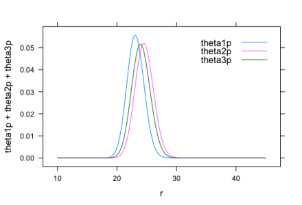
And similarly for theta2 and theta3. The resulting posteriors are:
We now have a posterior distribution for for our Poisson model of accidents from 1976 to 1985, so we can simulate Poisson values based on the distribution of , and from these simulations we can answer the exercise’s question to find the 95% predictive interval for 1986. We do this by first sampling ‘s with R‘s sample function — using our distribution for as sample weights — then simulate:

rsim <- sample (r, 20000, replace=T, prob=theta3p)
sim.theta3p <- rpois (20000, rsim)

It’s now a simple issue of taking the appropriate quantile:

quantile (sim.theta3p, c(0.025, 0.975))

and the answer is [15, 35], which basically agrees with the answer from the book’s website ([14, 35]). We could have, of course, taken the mean (24.0) or the calculated the standard deviation (5.1), or done any other kind of calculation on the resulting simulated values, which is the beauty of simulation (Monte Carlo) methods.

So, to summarize: we used only Bayes Rule, simulation, and the Poisson density and random numbers (dpois and rpois, respectively) to analyze some data using Bayesian techniques. No other distributions, no hyperparameters or parametric priors, no MCMC libraries. Just plain and simple (naive) work from first principles.

There are several issues to investigate further, including:

• All of the multiplications I’m doing will lose precision. How to avoid that?
• How important is normalization?
• The posterior distribution looks Gaussian: is it?
• Can we match a parametric density to sim.val?
• What if we’d used and maintained parametric distributions throughout the process?
• And (related to the previous point), what about that conjugate prior issue?

I’ll start down this list in my next entry.

[1] Bayesian Data Analysis, 2nd ed, 2004 by Gelman, Carlin, Stern, and Rubin