Deep Learning Dude pt 1

You’ve probably noticed that Deep Learning is all the rage right now. AlphaGo has beaten the world champion at Go, you can google cat photos and be sure you won’t accidentally get photos of canines, and many other near-miraculous feats: all enabled by Deep Learning with neural nets. (I am thinking of coining the phrase “laminar learning” to add some panache to old-school non-deep learning.)

I do a lot of my work in R, and it turns out that not one but two R packages have recently been released that enable R users to use the famous Python-based deep learning package, Keras: keras and kerasR.

model2

Continue reading

Donoho nails Data Science! Mostly.

Just a quick note: In his recent (when I wrote this but neglected to publish it) paper, 50 Years of Data Science, David Donaho pretty much nails key foundations of Data Science and how it’s different from (just) Statistics or even (just) Machine Learning. I highly recommend that you read it.

It’s full of great quotes like this:

“… In those less-hyped times, the skills being touted today were unnecessary. Instead, scientists developed skills to solve the problem they were really interested in, using elegant mathematics and powerful quantitative programming environments modeled on that math. Those environments were the result of 50 or more years of continual refinement, moving ever closer towards the ideal of enabling immediate translation of clear abstract thinking to computational results.

“The new skills attracting so much media attention are not skills for better solving the real problem of inference from data; they are coping skills for dealing with organizational artifacts of large-scale cluster computing. …”

Great stuff.

R Users Will Now Inevitably Become Bayesians

There are several reasons why everyone isn’t using Bayesian methods for regression modeling. One reason is that Bayesian modeling requires more thought: you need pesky things like priors, and you can’t assume that if a procedure runs without throwing an error that the answers are valid. A second reason is that MCMC sampling — the bedrock of practical Bayesian modeling — can be slow compared to closed-form or MLE procedures. A third reason is that existing Bayesian solutions have either been highly-specialized (and thus inflexible), or have required knowing how to use a generalized tool like BUGS, JAGS, or Stan. This third reason has recently been shattered in the R world by not one but two packages: brms and rstanarm. Interestingly, both of these packages are elegant front ends to Stan, via rstan and shinystan.

This article describes brms and rstanarm, how they help you, and how they differ.

BRMS Diagnostic 1
Continue reading

Real Data Science pt1: Review of Numbersense

So far, when I’ve written on Data Science topics I’ve written about the fun part: the statistical analysis, graphs, conclusions, insights, etc. For this next series of postings, I’m going to concentrate more on what we can call Real Data Science®: the less glamorous side of the job, where you have to beat your data and software into submission, where you don’t have access to the tools or data you need, and so on. In other words, where you spend the vast majority of your time as a Data Scientist.

I’ll start the series with a review of Kaiser Fung’s Numbersense, published in 2013. It’s not mainly about Real Data Science, but I’ll start with it because it’s a great book that illustrate several common data pitfalls, and in the epilogue Kaiser shares one of his own Real Data Science stories and I found myself nodding my head and saying, “Yup, that’s how I spent several days in the last couple of weeks!”

IMG_1078
Continue reading

Book recommendation: Longitudinal Structural Equation Modeling

Longitudinal Structural Equation Modeling, Todd D. Little, Guilford Press 2013.

Let me start by saying that this is one of the best textbooks I’ve ever read. It was written as if the author was our mentor, and I really get the feeling that he’s sharing his wisdom with us rather than trying to be pedagogically correct. The book is full of insights on how he thinks about building and applying SEMs, and the lessons he’s learned the hard way.

LittleBook
Continue reading

Constraint Programming tool advice?

I’m working on a scheduling project and have so far been using linear programming tools. As I look down the road, I’m beginning to think that I’ll need to supplement or move beyond LP, perhaps with something like constraint programming (CP) techniques. Unfortunately, the CP arena seems to be littered with tools that are highly-spoken of but are no longer (or barely) supported. Anyone out there who can address CP tools?

So far, I’m leaning towards OscaR, because it seems fairly complete and it’s in Scala which is the Official General-Purpose Language of Thinkinator. I’ve looked at a variety of CP tools like Zinc (seems dead) and MiniZinc (seems barely alive), Geocode (C++), JaCoP (java-based), Choco (java-based), Comet (seems dead), etc. It’s a bit worrisome when I compare the level of activity and the apparent long-term stability of these projects to linear programming (Symphony, glpsol, lpsolv, etc).

Any experiences or insights on CP tools? (I’d prefer standalone tools with high-level syntax or Scala/Java-based tools, and not C++/Prolog-based tools.) Thanks!

Where’s the Magic? (EMD and SSA in R)

When I first heard of SSA (Singular Spectrum Analysis) and the EMD (Empirical Mode Decomposition) I though surely I’ve found a couple of magical methods for decomposing a time series into component parts (trend, various seasonalities, various cycles, noise). And joy of joys, it turns out that each of these methods is implemented in R packages: Rssa and EMD.

In this posting, I’m going to document some of my explorations of the two methods, to hopefully paint a more realistic picture of what the packages and the methods can actually do. (At least in the hands of a non-expert such as myself.)

spiro2
Continue reading

Three-month forecasts to monthly estimates

In a previous series of postings, I described a model that I developed to predict monthly electricity usage and expenditure for a condo association. I based my model on the average monthly temperature at a nearby NOAA weather station at Ronald Reagan Airport (DCA), because the results are reasonable and more importantly because I can actually obtain forecasts from NOAA up to a year out.

The small complication is that the NOAA forecasts cover three-month periods rather than single month: JFM (Jan-Feb-Mar), FMA (Feb-Mar-Apr), MAM (Mar-Apr-May), etc. So, in this posting, we’ll briefly describe how to turn a series of these overlapping three-month forecasts into a series of monthly approximations.

temps3temps1
Continue reading

Electricity Usage in a High-rise Condo Complex pt 6 (discussion of model)

In Part 4 of this series, I created a Bayesian model in Stan. A member of the Stan team, Bob Carpenter, has been so kind as to send me some comments via email, and has given permission to post them on the blog. This is a great opportunity to get some expert insights! I’ll put his comments as block quotes:

That’s a lot of iterations! Does the data fit the model well?

I hadn’t thought about this. Bob noticed in both the call and the summary results that I’d run Stan for 300,000 iterations, and it’s natural to wonder, “Why so many iterations? Was it having trouble converging? Is something wrong?” The stan command defaults to four chains, each with 2,000 iterations, and one of the strengths of Stan‘s HMC algorithm is that the iterations are a bit slower than other methods but it mixes much faster so you don’t need nearly as many iterations. So 300,000 is a bit excessive. It turns out that if I run for 2,000 iterations, it takes 28 seconds on my laptop and mixes well. Most of the 28 seconds is taken up by compiling the model, since I can get 10,000 iterations in about 40 seconds.

So why 300,000 iterations? For the silly reason that I wanted lots of samples to make the CI’s in my plot as smooth as possible. Stan is pretty fast, so it only took a few minutes, but I hadn’t thought of implication of appearing to need that many iterations to converge.

stan1
Continue reading

Electricity Usage in a High-rise Condo Complex pt 5

Last time, we modeled the Association’s electricity expenditure using Bayesian Analysis. Besides the fact that MCMC and Bayesian are sexy and resume-worthy, what have we gained by using Stan? MCMC runs more slowly than alternatives, so it had better be superior in other ways, and in this posting, we’ll look at an example of how. I’d recommend pulling the previous posting up in another browser window or tab, and position the “Inference for Stan model” table so that you can quickly consult it in the following discussion.

If you look closely at the numbers, you may notice that the high season (warmer-high, ratetemp 3, beta[3]) appears to have a lower slope than the mid season (warmer-low, ratetemp 2, beta[2]), as was the case in an earlier model. This seems backwards: the high season should cost more per additional kWh, and thus should have a higher slope. This raises two questions: 1) is the apparent slope difference real, and 2) if it is real, is there some real-world basis for this counter-intuitive result?
Continue reading

New R-related website

There’s a new R-related website out there: Rdocumentation, which gathers the documentation for most R packages (that are hosted on CRAN) in one place and allows you to search through it.

There are a couple major benefits to the site:

  • It also provides a comments area where you can share thoughts, questions, and tips on various packages or even individual functions. (Though we’ll have to see if a critical mass builds for this.)
  • If you search in your own R installation with ?? you will only search the packages you have installed. I’m a package junkie, so have a huge number installed, but it’s still nice to have a place where I can discover new packages more easily.

So check it out and make suggestions to the creators. This should really be rolled into CRAN at some point.

Electricity Usage in a High-rise Condo Complex pt 4

This is the fourth article in the series, where the techiness builds to a crescendo. If this is too statistical/programming geeky for you, the next posting will return to a more investigative and analytical flavor. Last time, we looked at a fixed-effects model:

m.fe <- lm (dollars ~ 1 + regime + ratetemp * I(dca - 55))

which looks like a plausible model and whose parameters are all statistically significant. A question that might arise is: why not use a hierarchical (AKA multilevel, mixed-effects) model instead? While we’re at it, why not go full-on Bayesian as well? It just so happens that there is a great new tool called Stan which fits the bill and which also has an rstan package for R.

stan1
Continue reading

Models, Statistical Significance, Actual Significance

“Sometimes people think that if a coefficient estimate is not significant, then it should be excluded from the model. We disagree. It is fine to have nonsignificant coefficients in a model, as long as they make sense.” Gelman & Hill 2007, page 42

“Include all variables that, for substantive reasons, might be expected to be important.” Ibid, page 69.

When a field adopts a common word and uses it in a technical sense, it’s sometimes lucky and sometimes unlucky.
Continue reading

Electricity Usage in a High-rise Condo Complex pt 3

In a previous installment, we looked at modeling electricity usage for the infrastructure and common areas of a condo association, and a fairly simple model was reasonably accurate. This makes sense in a large system such as mid-sized, high-rise condo building, which has a lot of electricity-usage inertia. The cost of that electricity has a lot more variability, however, because of rate changes (increases and decreases), refunds, high/low seasons, and other factors that affect the bottom line.

FE1 Continue reading

Electricity Usage in a High-rise Condo Complex pt 2

In a previous installment, we described a condo association that needed to know what its electricity budget should be for an upcoming budget. In this posting, we’ll develop a model for electricity utilization, leaving electricity expenses for the next installment.

I like to have pretty pictures above the fold, so let’s take a look at the data and the resulting model, all in one convenient and colorful graph. The graph shows each month’s average daily electricity usage (in kilowatt hours, kWh) versus the month’s average temperature at nearby Ronald Reagan Airport (DCA). Each month’s bill is a point at the center of the month name:

Figure 1: Average Daily electricity usage by temperature Continue reading

Electricity Usage in a High-rise Condo Complex pt 1

This is the story of a condominium association in Northern Virginia, which was in the midst of transforming their budget. In the early days of the association they didn’t have an operational cash reserve built up, so they had to make budget categories a bit oversized, “just in case”. As time went on, they saved the cash from their over-estimates, and eventually arrived at the place where they could set tighter budgets and depend on their cash savings if the budget were exceeded.

In the process of reviewing various categories, they came to “Utilities”, which lumped water, sewage, gas, and electricity all together. They decided to break it down into individual utilities, but when they started with electricity, no one actually knew how much was used nor how much it cost. The General Manager had dutifully filed away monthly bills from Dominion, but didn’t have a spreadsheet. They needed a data analyst, and I was all over it.

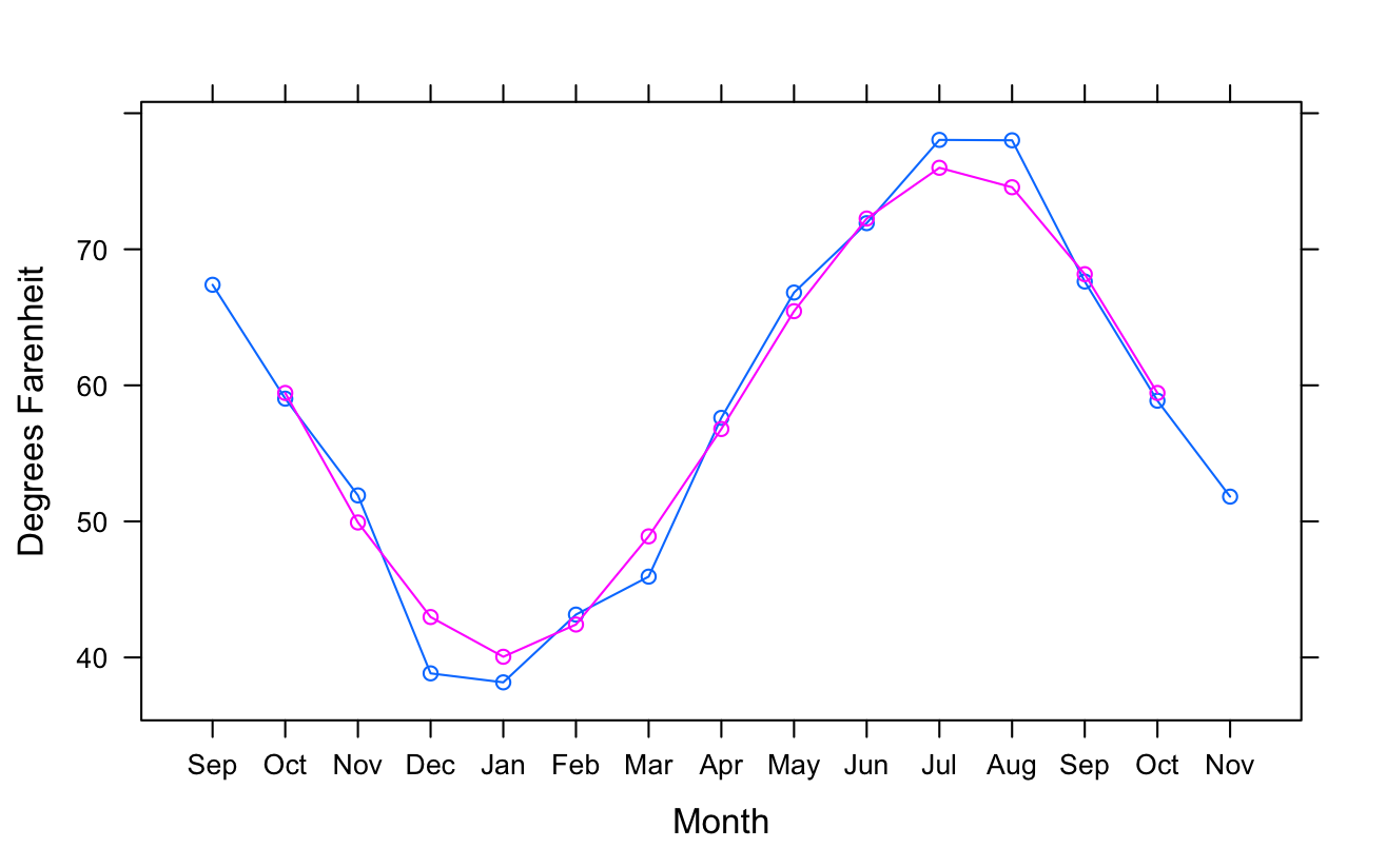
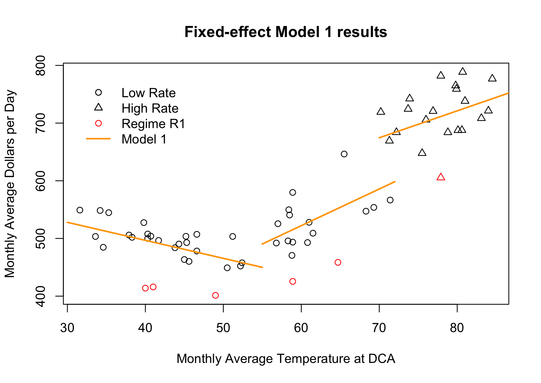
In the next four or five postings, I want to show some of the details of my investigation of electricity expenses. I hope it will be an interesting look at the kinds of things that happen in the real world, not just textbooks. Oh, by the way, it turns out that electricity was the single largest operating expense of the association. Here’s a graph of average expenditures, brought up to the present:

Initial Graph Continue reading

Automatic Report Generation in R, with knitr and markdown

This is a quick introduction to using R, the R package `knitr`, and the markdown language to automatically generate monthly reports.

Let’s say I track electricity usage and expenses for a client. I initially spent a lot of time analyzing and making models for the data, but at this point I’m now in more of a maintenance mode and simply want an updated report to email each month. So, when their new electricity bill arrives I scrape the data into R, save the data in an R workspace, and then use knitr to generate a simplistic HTML report.

Continue reading

It’s the Little Differences That Matter

Everyone’s interested in the global climate these days, so I’ve been looking at the GISTEMP temperature series, from the GISS (NASA’s Goddard Institute for Space Studies). I was recently analyzing the data and it turned into an interesting data forensics operation that I hope will inspire you to dig a little deeper into your data.

Let’s start with the data. GISS has a huge selection of data for the discerning data connoisseur, so which to choose? The global average seems too coarse — the northern and southern hemispheres are out of phase and dominated by different geography. On the other hand, the gridded data is huge and requires all kinds of spatially-saavy processing to be useful. (We may go there in a future post, but not today.) So let’s start with the two hemisphere monthly average datasets, which I’ll refer to as GISTEMP NH and GISTEMP SH.

To be specific, these time series are GISTEMP LOTI (Land Ocean Temperature Index) which means that they cover both land and sea. GISS has land-only data and combines this with NOAA’s sea-only data from ERSST (Extended Reconstructed Sea Surface Temperature). I’d also point out that all of the temperature data I’ll use is measured as an anomaly from the average temperature over the years 1951-1980, which was approximately 14 degrees Celsius (approximately 57 degrees Farenheit). So let’s plot the GISTEMP LOTI NH and SH data and see what we have.

1 GISTEMP series

Continue reading