In a previous installment, we looked at modeling electricity usage for the infrastructure and common areas of a condo association, and a fairly simple model was reasonably accurate. This makes sense in a large system such as mid-sized, high-rise condo building, which has a lot of electricity-usage inertia. The cost of that electricity has a lot more variability, however, because of rate changes (increases and decreases), refunds, high/low seasons, and other factors that affect the bottom line.

So an expenditure model will need to be more complex than a usage model to account for at least some of these additional issues. I did some initial investigation of external factors such as energy prices, but with the diversification of Dominion’s fuels, energy price lags, the lags inherent in the rate-change process, etc, that didn’t yield anything useful. We know when major billing changes occurred, so I created a regime indicator which has five regimes between changes, R1 … R5, where the most important distinction is that between R1 and R2 there was a 20%+ increase which hasn’t been matched since. We also know that rates are higher in June through September, so I created a rate indicator which is high for June-Sep and low for other months.

Note that for any particular month rate is the same across years, while temp can be different. (Though, realistically, only for fall/spring months: we’re not going to see an August that averages cooler than 55 degrees.) As you look at some of the following graphs with dca in them, keep in mind that temp has a specific boundary (55 degrees), while rate does not. There’s a soft boundary somewhere around 70-72 degrees, but it it’s only approximate.

For convenience, I created another indicator, ratetemp, which combines rate (higher and lower) and temp (warmer than 54 degrees and cooler than 54 degrees), but actually only has three values since the combination high-cooler isn’t realistically possible.

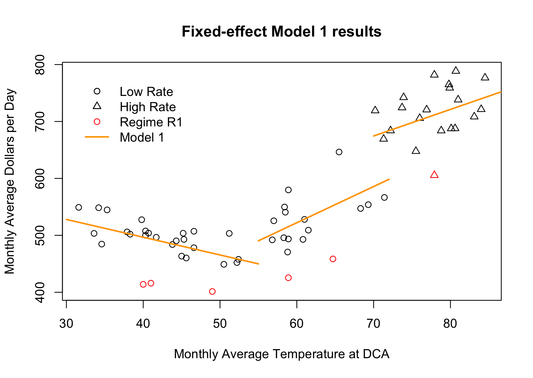
So what would a motivated regression look like? A first cut, using fixed-effects might be:

m.fe <- lm (dollars ~ 1 + regime + ratetemp * I(dca - 55))

which is visualized in the graph, above.

The lines might not appear to be well-placed, and there is a reason for that. The points on the graph cover all five regimes, but the lines illustrate the current model fit, in regime R5. The extra-low R1 points are marked in red, for example. What else stands out in the graph?

First, there’s a jump at 55 degrees that did not appear in the usage model. One explanation for this is that there is a jump in demand in the Spring, perhaps when the cooling towers are turned on. We’ll talk about demand in an upcoming part of this series; it’s one of the significant findings of my investigation.

Second, the high-warmer segment actually has a lower slope (4.7) than the low-warmer segment (6.4), whereas the rates being charged are higher which should create a higher slope. One explanation for this is that the tariff’s cost for each additional kWh of electricity decreases as usage increases, with the bottom tier being 16x more expensive than the top tier. We’ll look at this in more detail when we discuss demand in a future posting. In the next posting, we’ll go full-on techie with a hierarchical Bayesian model of expenditures.