BRMS continues its streak

As you probably know, I’m a big fan of R’s brms package, available from CRAN. In case you haven’t heard of it, brms is an R package by Paul-Christian Buerkner that implements Bayesian regression of all types using an extension of R’s formula specification that will be familiar to users of lm, glm, and lmer. Under the hood, it translates the formula into Stan code, Stan translates this to C++, your system’s C++ compiler is used to compile the result and it’s run.

screen-shot-2016-11-20-at-4-38-05-pm

brms is impressive in its own right. But also impressive is how it continues to add capabilities and the breadth of Buerkner’s vision for it. I last posted something way back on version 0.8, when brms gained the ability to do non-linear regression, but now we’re up to version 1.1, with 1.2 around the corner. What’s been added since 0.8, you may ask? Here are a few highlights:

Continue reading

Advertisement

R Users Will Now Inevitably Become Bayesians

There are several reasons why everyone isn’t using Bayesian methods for regression modeling. One reason is that Bayesian modeling requires more thought: you need pesky things like priors, and you can’t assume that if a procedure runs without throwing an error that the answers are valid. A second reason is that MCMC sampling — the bedrock of practical Bayesian modeling — can be slow compared to closed-form or MLE procedures. A third reason is that existing Bayesian solutions have either been highly-specialized (and thus inflexible), or have required knowing how to use a generalized tool like BUGS, JAGS, or Stan. This third reason has recently been shattered in the R world by not one but two packages: brms and rstanarm. Interestingly, both of these packages are elegant front ends to Stan, via rstan and shinystan.

This article describes brms and rstanarm, how they help you, and how they differ.

BRMS Diagnostic 1
Continue reading

Book recommendation: Longitudinal Structural Equation Modeling

Longitudinal Structural Equation Modeling, Todd D. Little, Guilford Press 2013.

Let me start by saying that this is one of the best textbooks I’ve ever read. It was written as if the author was our mentor, and I really get the feeling that he’s sharing his wisdom with us rather than trying to be pedagogically correct. The book is full of insights on how he thinks about building and applying SEMs, and the lessons he’s learned the hard way.

LittleBook
Continue reading

Three-month forecasts to monthly estimates

In a previous series of postings, I described a model that I developed to predict monthly electricity usage and expenditure for a condo association. I based my model on the average monthly temperature at a nearby NOAA weather station at Ronald Reagan Airport (DCA), because the results are reasonable and more importantly because I can actually obtain forecasts from NOAA up to a year out.

The small complication is that the NOAA forecasts cover three-month periods rather than single month: JFM (Jan-Feb-Mar), FMA (Feb-Mar-Apr), MAM (Mar-Apr-May), etc. So, in this posting, we’ll briefly describe how to turn a series of these overlapping three-month forecasts into a series of monthly approximations.

temps3temps1
Continue reading

Fun with R and HMM’s

I’m always intrigued by techniques that have cool names: Support Vector Machines, State Space Models, Spectral Clustering, and an old favorite Hidden Markov Models (HMM’s). While going through some of my notes, I stumbled onto a fun experiment with HMM’s where you feed a bunch of English text into a two-state HMM and it will (tend to) discover what letters are vowels.
bw1
Continue reading

Stata for R users pt 1

I did a quick Google search on “Stata for R users” (both as separate words and as a quoted phrase) and there really isn’t much out there. At best, there are a couple of equivalence guides that show you how to do certain tasks in both programs. (Plus a whole lot of “R for (ex-) Stata users” articles.) I’m writing this post, as a long-term R user who recently bought Stata, because I believe that Stata is a good complement to R, and many R users should consider adding it to their toolbox.

I’m going to write this in two parts. Part one will describe why an R user might be interested in Stata — with various Stata examples. Part Two will give specific tips and warnings to R users who do decide to use Stata.
Stata 13 logo Continue reading

Stata 13 is nice

I’m a big fan of R, and it will be my primary tool for a long time, but I wanted to add another tool to my toolbox and decided on Stata. Stata 13 was just released (June 2013), and I have to say that it’s a very nice package.

Why would anyone pick Stata over R? R has many advantages, but here are some reasons that you might pick Stata:
Continue reading

Electricity Usage in a High-rise Condo Complex pt 6 (discussion of model)

In Part 4 of this series, I created a Bayesian model in Stan. A member of the Stan team, Bob Carpenter, has been so kind as to send me some comments via email, and has given permission to post them on the blog. This is a great opportunity to get some expert insights! I’ll put his comments as block quotes:

That’s a lot of iterations! Does the data fit the model well?

I hadn’t thought about this. Bob noticed in both the call and the summary results that I’d run Stan for 300,000 iterations, and it’s natural to wonder, “Why so many iterations? Was it having trouble converging? Is something wrong?” The stan command defaults to four chains, each with 2,000 iterations, and one of the strengths of Stan‘s HMC algorithm is that the iterations are a bit slower than other methods but it mixes much faster so you don’t need nearly as many iterations. So 300,000 is a bit excessive. It turns out that if I run for 2,000 iterations, it takes 28 seconds on my laptop and mixes well. Most of the 28 seconds is taken up by compiling the model, since I can get 10,000 iterations in about 40 seconds.

So why 300,000 iterations? For the silly reason that I wanted lots of samples to make the CI’s in my plot as smooth as possible. Stan is pretty fast, so it only took a few minutes, but I hadn’t thought of implication of appearing to need that many iterations to converge.

stan1
Continue reading

Electricity Usage in a High-rise Condo Complex pt 5

Last time, we modeled the Association’s electricity expenditure using Bayesian Analysis. Besides the fact that MCMC and Bayesian are sexy and resume-worthy, what have we gained by using Stan? MCMC runs more slowly than alternatives, so it had better be superior in other ways, and in this posting, we’ll look at an example of how. I’d recommend pulling the previous posting up in another browser window or tab, and position the “Inference for Stan model” table so that you can quickly consult it in the following discussion.

If you look closely at the numbers, you may notice that the high season (warmer-high, ratetemp 3, beta[3]) appears to have a lower slope than the mid season (warmer-low, ratetemp 2, beta[2]), as was the case in an earlier model. This seems backwards: the high season should cost more per additional kWh, and thus should have a higher slope. This raises two questions: 1) is the apparent slope difference real, and 2) if it is real, is there some real-world basis for this counter-intuitive result?
Continue reading

Electricity Usage in a High-rise Condo Complex pt 4

This is the fourth article in the series, where the techiness builds to a crescendo. If this is too statistical/programming geeky for you, the next posting will return to a more investigative and analytical flavor. Last time, we looked at a fixed-effects model:

m.fe <- lm (dollars ~ 1 + regime + ratetemp * I(dca - 55))

which looks like a plausible model and whose parameters are all statistically significant. A question that might arise is: why not use a hierarchical (AKA multilevel, mixed-effects) model instead? While we’re at it, why not go full-on Bayesian as well? It just so happens that there is a great new tool called Stan which fits the bill and which also has an rstan package for R.

stan1
Continue reading

Models, Statistical Significance, Actual Significance

“Sometimes people think that if a coefficient estimate is not significant, then it should be excluded from the model. We disagree. It is fine to have nonsignificant coefficients in a model, as long as they make sense.” Gelman & Hill 2007, page 42

“Include all variables that, for substantive reasons, might be expected to be important.” Ibid, page 69.

When a field adopts a common word and uses it in a technical sense, it’s sometimes lucky and sometimes unlucky.
Continue reading

Electricity Usage in a High-rise Condo Complex pt 3

In a previous installment, we looked at modeling electricity usage for the infrastructure and common areas of a condo association, and a fairly simple model was reasonably accurate. This makes sense in a large system such as mid-sized, high-rise condo building, which has a lot of electricity-usage inertia. The cost of that electricity has a lot more variability, however, because of rate changes (increases and decreases), refunds, high/low seasons, and other factors that affect the bottom line.

FE1 Continue reading

Electricity Usage in a High-rise Condo Complex pt 2

In a previous installment, we described a condo association that needed to know what its electricity budget should be for an upcoming budget. In this posting, we’ll develop a model for electricity utilization, leaving electricity expenses for the next installment.

I like to have pretty pictures above the fold, so let’s take a look at the data and the resulting model, all in one convenient and colorful graph. The graph shows each month’s average daily electricity usage (in kilowatt hours, kWh) versus the month’s average temperature at nearby Ronald Reagan Airport (DCA). Each month’s bill is a point at the center of the month name:

Figure 1: Average Daily electricity usage by temperature Continue reading

Electricity Usage in a High-rise Condo Complex pt 1

This is the story of a condominium association in Northern Virginia, which was in the midst of transforming their budget. In the early days of the association they didn’t have an operational cash reserve built up, so they had to make budget categories a bit oversized, “just in case”. As time went on, they saved the cash from their over-estimates, and eventually arrived at the place where they could set tighter budgets and depend on their cash savings if the budget were exceeded.

In the process of reviewing various categories, they came to “Utilities”, which lumped water, sewage, gas, and electricity all together. They decided to break it down into individual utilities, but when they started with electricity, no one actually knew how much was used nor how much it cost. The General Manager had dutifully filed away monthly bills from Dominion, but didn’t have a spreadsheet. They needed a data analyst, and I was all over it.

In the next four or five postings, I want to show some of the details of my investigation of electricity expenses. I hope it will be an interesting look at the kinds of things that happen in the real world, not just textbooks. Oh, by the way, it turns out that electricity was the single largest operating expense of the association. Here’s a graph of average expenditures, brought up to the present:

Initial Graph Continue reading

It’s the Little Differences That Matter

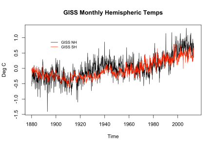
Everyone’s interested in the global climate these days, so I’ve been looking at the GISTEMP temperature series, from the GISS (NASA’s Goddard Institute for Space Studies). I was recently analyzing the data and it turned into an interesting data forensics operation that I hope will inspire you to dig a little deeper into your data.

Let’s start with the data. GISS has a huge selection of data for the discerning data connoisseur, so which to choose? The global average seems too coarse — the northern and southern hemispheres are out of phase and dominated by different geography. On the other hand, the gridded data is huge and requires all kinds of spatially-saavy processing to be useful. (We may go there in a future post, but not today.) So let’s start with the two hemisphere monthly average datasets, which I’ll refer to as GISTEMP NH and GISTEMP SH.

To be specific, these time series are GISTEMP LOTI (Land Ocean Temperature Index) which means that they cover both land and sea. GISS has land-only data and combines this with NOAA’s sea-only data from ERSST (Extended Reconstructed Sea Surface Temperature). I’d also point out that all of the temperature data I’ll use is measured as an anomaly from the average temperature over the years 1951-1980, which was approximately 14 degrees Celsius (approximately 57 degrees Farenheit). So let’s plot the GISTEMP LOTI NH and SH data and see what we have.

1 GISTEMP series

Continue reading

Bayesian Data Analysis 3

In the first posting of this series, I simply applied Bayes Rule repeatedly: Posterior \propto Prior \times Likelihood. I didn’t have to know anything about conjugate priors, hyperparameters, sufficient statistics, parametric forms, or anything beyond the basics. I got a reasonable posterior for \theta and used that to find the correct answer. Why go beyond this?

Well, first, there’s really no good way for me to communicate my \theta distribution to anyone else. It’s a (long) vector of values, and that’s the weakness of a non-parametric system: there is no well-known function and no sufficient statistics to easily describe what I’ve discovered. (Of course, it’s possible that there is no well-know function that’s appropriate, in which case the simulation method is actually the only option.)

Second, my posterior density is discrete. This works reasonably well for the exercise I attempted, but it’s still a discrete approximation which is less precise and can suffer from simulation-related issues (number of samples, etc) that have nothing to do with my proposed model.

Third, if an analytical method can be used, it may be possible to directly calculate a final posterior without repeated applications of Bayes Rule. As I mentioned in the previous posting, Gelman got an answer of Gamma(238, 10) analytically, not through approximations and simulation. If we look in Wikipedia, we can find that the conjugate prior for \theta, the parameter of a Poisson distribution, is the Gamma (\alpha, \beta) distribution, and given our series of n accident counts and an initial (posterior) \alpha and \beta, the posterior density is Gamma (\alpha - \sum_{i=1}^{n} \mathrm {accident}_i, \beta + n)

Continue reading

Bayesian Data Analysis 2

In the last post (Bayesian Data Analysis 1), I ran a Bayesian data analysis using a simple, first-principles approach. Armed with only the fact that a Poisson distribution is appropriate for modeling airplane accidents, Bayes Rule, and R, we got the correct answer to the problem through non-parametric simulation.

Before we get into precision and the other topics in the list of issues to explore, let’s tie up one loose end. I could have gotten the right answer for the wrong reason, so let’s look at the posterior distribution of \theta as compared to the provided answer to make sure we’re close. In the answer, Gelman looks at the parametrical form for \theta and considers conjugate priors and analytically determines that the correct parametric posterior distribution is a Gamma function with \alpha=238 and \beta=10. (More on this in the next posting.) So I simulated out 20,000 samples from that distribution:

rgam <- rgamma (20000, 238, 10)

And then we can compare our posterior distribution with the official, parametric distribution:

Looks reasonably close (though biased by about 0.25) and it didn’t take a lot of fancy machinery to pull off. So why not use this method as our default? Why talk of things like conjugate priors and hyper parameters? And did we just get lucky with numeric precision because we only had 10 accidents and hence only 10 applications of Bayes Rule? Let’s cover that in the next posting, and finish this one with a graph of our answer (not \theta but the predictive distribution of accidents) with the 95% CI :

Bayesian Data Analysis 1

I’ve read quite a few presentations on Bayesian data analysis, but I always seem to fall into the crack between the first, one-step problem (the usual being how likely you are to have a disease), and more advanced problems that involve conjugate priors and quite a few other concepts. So, when I was recently reading Bayesian Data Analysis[1], I decided to tackle Exercise 13 from Chapter 2 using only Bayes rule updates and simulation. I think it’s been illuminating, so decided to write it up here, using my favorite tool R.

Exercise 13 involves annual airline accidents from 1976 to 1985, modeled as a Poisson(\theta) distribution. The data is :

accidents <- c(24, 25, 31, 31, 22, 21, 26, 20, 16, 22)

A little playing around with graphs and R‘s dpois gives me the impression that \theta is probably around 24, but I’ll make three priors (for \theta):

r <- seq (10, 45, 0.2)
theta1 <- dnorm (r, 15, 5)
theta1 <- theta1 / sum (theta1)
theta2 <- dnorm (r, 35, 6)
theta2 <- theta2 / sum (theta2)
theta3 <- 20 - abs (r - mean (r))
theta3 <- theta3 / sum (theta3)

Where theta1 is probably low, theta2 is probably high, and theta3 is not even parametric. (More on this later.) I normalized them to create proper priors so that they graph well together, but that wasn’t necessary. Remember, I’m doing all of my calculations over the discretized range, r. Plotting the theta’s together:

So let’s run the numbers (accidents) through a repeated set of Bayes Rule updates to get a posterior distribution for \theta based on the prior distribution, theta1:

Continue reading