There are several reasons why everyone isn’t using Bayesian methods for regression modeling. One reason is that Bayesian modeling requires more thought: you need pesky things like priors, and you can’t assume that if a procedure runs without throwing an error that the answers are valid. A second reason is that MCMC sampling — the bedrock of practical Bayesian modeling — can be slow compared to closed-form or MLE procedures. A third reason is that existing Bayesian solutions have either been highly-specialized (and thus inflexible), or have required knowing how to use a generalized tool like BUGS, JAGS, or Stan. This third reason has recently been shattered in the R world by not one but two packages: brms and rstanarm. Interestingly, both of these packages are elegant front ends to Stan, via rstan and shinystan.
This article describes brms and rstanarm, how they help you, and how they differ.
You can install both packages from CRAN, making sure to install dependencies so you get rstan, Rcpp, and shinystan as well. [EDIT: Note that you will also need a C++ compiler to make this work, as Charles and Paul Bürkner (@paulbuerkner) have found. On Windows that means you’ll need to install Rtools, and on the Mac you may have to install Xcode (which is also free). brms‘s help refers to the RStan Getting Started, which is very helpful.] If you like having the latest development versions — which may have a few bug fixes that the CRAN versions don’t yet have — you can use devtools to install them following instructions at the brms github site or the rstanarm github site.
The brms package
Let’s start with a quick multinomial logistic regression with the famous Iris dataset, using brms. You may want to skip the actual brm call, below, because it’s so slow (we’ll fix that in the next step):
library (brms)

rstan_options (auto_write=TRUE)
options (mc.cores=parallel::detectCores ()) # Run on multiple cores

set.seed (3875)

ir <- data.frame (scale (iris[, -5]), Species=iris[, 5])

### With improper prior it takes about 12 minutes, with about 40% CPU utilization and fans running,
### so you probably don't want to casually run the next line...

system.time (b1 <- brm (Species ~ Petal.Length + Petal.Width + Sepal.Length + Sepal.Width, data=ir,
                        family="categorical", n.chains=3, n.iter=3000, n.warmup=600))
First, note that the brm call looks like glm or other standard regression functions. Second, I advised you not to run the brm because on my couple-of-year-old Macbook Pro, it takes about 12 minutes to run. Why so long? Let’s look at some of the results of running it:
b1 # ===> Result, below

 Family: categorical (logit)
Formula: Species ~ Petal.Length + Petal.Width + Sepal.Length + Sepal.Width
   Data: ir (Number of observations: 150)
Samples: 3 chains, each with n.iter = 3000; n.warmup = 600; n.thin = 1;
         total post-warmup samples = 7200
   WAIC: NaN

Fixed Effects:
                Estimate Est.Error  l-95% CI u-95% CI Eff.Sample Rhat
Intercept[1]     1811.49   1282.51   -669.27  4171.99         16 1.26
Intercept[2]     1773.48   1282.87   -707.92  4129.22         16 1.26
Petal.Length[1]  3814.69   6080.50  -8398.92 15011.29          2 2.32
Petal.Length[2]  3848.02   6080.70  -8353.52 15032.85          2 2.32
Petal.Width[1]  14769.65  18021.35  -2921.08 54798.11          2 3.36
Petal.Width[2]  14794.32  18021.10  -2902.81 54829.05          2 3.36
Sepal.Length[1]  1519.97   1897.12  -2270.30  5334.05          7 1.43
Sepal.Length[2]  1515.83   1897.17  -2274.31  5332.95          7 1.43
Sepal.Width[1]  -7371.98   5370.24 -18512.35  -935.85          2 2.51
Sepal.Width[2]  -7377.22   5370.22 -18515.78  -941.65          2 2.51
A multinomial logistic regression involves multiple pair-wise logistic regressions, and the default is a baseline level versus the other levels. In this case, the last level (virginica) is the baseline, so we see results for 1) setosa v virginica, and 2) versicolor v virginica. (brms provides three other options for ordinal regressions, too.)
The first “diagnostic” we might notice is that it took way longer to run than we might’ve expected (12 minutes) for such a small dataset. Turning to the formal results above, we see huge estimated coefficients, huge error margins, a tiny effective sample size (2-16 effective samples out of 7200 actual samples), and an Rhat significantly different from 1. So we can officially say something (everything, actually) is very wrong.
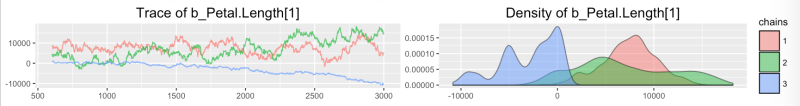
If we were coding in Stan ourselves, we’d have to think about bugs we might’ve introduced, but with brms, we can assume for now that the code is correct. So the first thing that comes to mind is that the default flat (improper) priors are so broad that the sampler is wandering aimlessly, which gives poor results and takes a long time because of many rejections. The first graph in this posting was generated by plot (b1), and it clearly shows non-convergence of Petal.Length[1] (setosa v virginica). This is a good reason to run multiple chains, since you can see how poor the mixing is and how different the densities are. (If we want nice interactive interface to all of the results, we could launch_shiny (b1).)
Let’s try again, with more reasonable priors. In the case of a logistic regression, the exponentiated coefficients reflect the increase in probability for a unit increase of the variable, so let’s try using a normal (0, 8) prior, (95% CI is 
system.time (b2 <- brm (Species ~ Petal.Length + Petal.Width + Sepal.Length + Sepal.Width), data=ir,
                        family="categorical", n.chains=3, n.iter=3000, n.warmup=600,
                        prior=c(set_prior ("normal (0, 8)"))))
This only takes about a minute to run — about half of which involves compiling the model in C++ — which is a more reasonable time, and the results are much better:
 Family: categorical (logit)
Formula: Species ~ Petal.Length + Petal.Width + Sepal.Length + Sepal.Width
   Data: ir (Number of observations: 150)
Samples: 3 chains, each with iter = 3000; warmup = 600; thin = 1;
         total post-warmup samples = 7200
   WAIC: 21.87

Fixed Effects:
                Estimate Est.Error l-95% CI u-95% CI Eff.Sample Rhat
Intercept[1]        6.90      3.21     1.52    14.06       2869    1
Intercept[2]       -5.85      4.18   -13.97     2.50       2865    1
Petal.Length[1]     4.15      4.45    -4.26    12.76       2835    1
Petal.Length[2]    15.48      5.06     5.88    25.62       3399    1
Petal.Width[1]      4.32      4.50    -4.50    13.11       2760    1
Petal.Width[2]     13.29      4.91     3.76    22.90       2800    1
Sepal.Length[1]     4.92      4.11    -2.85    13.29       2360    1
Sepal.Length[2]     3.19      4.16    -4.52    11.69       2546    1
Sepal.Width[1]     -4.00      2.37    -9.13     0.19       2187    1
Sepal.Width[2]     -5.69      2.57   -11.16    -1.06       2262    1
Much more reasonable estimates, errors, effective samples, and Rhat. And let’s compare a plot for Petal.Length[1]:
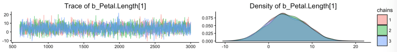
Ahhh, that looks a lot better. The chains mix well and seem to randomly explore the space, and the densities closely agree. Go back to the top graph and compare, to see how much of an influence poor priors can have.
We have a wide choice of priors, including Normal, Student’s t, Cauchy, Laplace (double exponential), and many others. The formula argument is a lot like lmer‘s (from package lme4, an excellent place to start a hierarchical/mixed model to check things before moving to Bayesian solutions) with an addition:
response | addition ~ fixed + (random | group)
where addition can be replaced with function calls se, weights, trials, cat, cens, or trunc, to specify SE of the observations (for meta-analysis), weighted regression, to specify the number of trials underlying each observation, the number of categories, and censoring or truncation, respectively. (See details of brm for which families these apply to, and how they are used.) You can do zero-inflated and hurdle models, specify multiplicative effects, and of course do the usual hierarchical/mixed effects (random and group) as well.
Families include: gaussian, student, cauchy, binomial, bernoulli, beta, categorical, poisson, negbinomial, geometric, gamma, inverse.gaussian, exponential, weibull, cumulative, cratio, sratio, acat, hurdle_poisson, hurdle_negbinomial, hurdle_gamma, zero_inflated_poisson, and zero_inflated_negbinomial. (The cratio, sratio, and acat options provide different options than the default baseline model for (ordinal) categorical models.)
All in one function! Oh, did I mention that you can specify AR, MA, and ARMA correlation structures?
The only downside to brms could be that it generates Stan code on the fly and passes it to Stan via rstan, which will result in it being compiled. For larger models, the 40-60 seconds for compilation won’t matter much, but for small models like this Iris model it dominates the run time. This technique provides great flexibility, as listed above, so I think it’s worth it.
Another example of brms‘ emphasis on flexibility is that the Stan code it generates is simple, and could be straightforwardly used to learn Stan coding or as a basis for a more-complex Stan model that you’d modify and then run directly via rstan. In keeping with this, brms provides the make_stancode and make_standata functions to allow direct access to this functionality.
The rstanarm package
The rstanarm package takes a similar, but different approach. Three differences stand out: First, instead of a single main function call, rstanarm has several calls that are meant to be similar to pre-existing functions you are probably already using. Just prepend with “stan_”: stan_lm, stan_aov, stan_glm, stan_glmer, stan_gamm4 (GAMMs), and stan_polr (Ordinal Logistic). Oh, and you’ll probably want to provide some priors, too.
Second, rstanarm pre-compiles the models it supports when it’s installed, so it skips the compilation step when you use it. You’ll notice that it immediately jumps to running the sampler rather than having a “Compiling C++” step. The code it generates is considerably more extensive and involved than the code brms generates, which seems to allow it to sample faster but which would also make it more difficult to take and adapt it by hand to go beyond what the rstanarm/brms approach offers explicitly. In keeping with this philosophy, there is no explicit function for seeing the generated code, though you can always look into the fitted model to see it. For example, if the model were br2, you could look at br2$stanfit@stanmodel@model_code.
Third, as its excellent vignettes emphasize, Bayesian modeling is a series of steps that include posterior checks, and rstanarm provides a couple of functions to help you, including pp_check. (This difference is not as hard-wired as the first two, and brms could/should someday include similar functions, but it’s a statement that’s consistent with the Stan team’s emphasis.)
As a quick example of rstanarm use, let’s build a (poor, toy) model on the mtcars data set:
mm  Results
stan_glm(formula = mpg ~ ., data = mtcars, prior = normal(0,
    8))

Estimates:
            Median MAD_SD
(Intercept) 11.7   19.1
cyl         -0.1    1.1
disp         0.0    0.0
hp           0.0    0.0
drat         0.8    1.7
wt          -3.7    2.0
qsec         0.8    0.8
vs           0.3    2.1
am           2.5    2.2
gear         0.7    1.5
carb        -0.2    0.9
sigma        2.7    0.4

Sample avg. posterior predictive
distribution of y (X = xbar):
         Median MAD_SD
mean_PPD 20.1    0.7
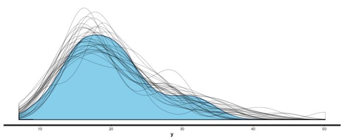
Note the more sparse output, which Gelman promotes. You can get more detail with summary (br), and you can also use shinystan to look at most everything that a Bayesian regression can give you. We can look at the values and CIs of the coefficients with plot (mm), and we can compare posterior sample distributions with the actual distribution with: pp_check (mm, "dist", nreps=30):
I could go into more detail, but this is getting a bit long, and rstanarm is a very nice package, too, so let’s wrap things up with a comparison of the two packages and some tips.
Commonalities and other differences
Both packages support a wide variety of regression models — pretty much everything you’ll ever need. Both packages use Stan, via rstan and shinystan, which means you can also use rstan capabilities as well, and you get parallel execution support — mainly useful for multiple chains, which you should always do. Both packages support sparse solutions, brms via Laplace or Horseshoe priors, and rstanarm via Hierarchical Shrinkage Family priors. Both packages support Stan 2.9’s new Variational Bayes methods, which are much faster then MCMC sampling (an order of magnitude or more), but approximate and only valid for initial explorations, not final results.
Because of its pre-compiled-model approach, rstanarm is faster in starting to sample for small models, and is slightly faster overall, though a bit less flexible with things like priors. brms supports (non-ordinal) multinomial logistic regression, several ordinal logistic regression types, and time-series correlation structures. rstanarm supports GAMMs (via stan_gamm4). rstanarm is done by the Stan/rstan folks. brms‘s make_stancode makes Stan less of a black box and allows you to go beyond pre-packaged capabilities, while rstanarm‘s pp_check provides a useful tool for the important step of posterior checking.
Summary
Bayesian modeling is a general machine that can model any kind of regression you can think of. Until recently, if you wanted to take advantage of this general machinery, you’d have to learn a general tool and its language. If you simply wanted to use Bayesian methods, you were often forced to use very-specialized functions that weren’t flexible. With the advent of brms and rstanarm, R users can now use extremely flexible functions from within the familiar and powerful R framework. Perhaps we won’t all become Bayesians now, but we now have significantly fewer excuses for not doing so. This is very exciting!
Stan tips
First, Stan’s HMC/NUTS sampler is slower per sample, but better explores the probability space, so you should be able to use fewer samples than you might’ve come to expect with other samplers. (Probably an order of magnitude fewer.) Second, Stan transforms code to C++ and then compiles the C++, which introduces an initial delay at the start of sampling. (This is bypassed in rstanarm.) Third, don’t forget the rstan_options and options statements I started with: you really need to run multiple chains and the fastest way to do that is by having Stan run multiple processes/threads.
Remember that the results of the stan_ plots, such as stan_dens or the results of rstanarm‘s plot (mod, "dens") are ggplot2 objects and can be modified with additional geoms. For example, if you want to zoom in on a density plot:
stan_plot (b2$fit, show_density=TRUE) + coord_cartesian (xlim=c(-15, 15))
(Note: you want to use coord_cartesian rather than xlim which eliminates points and screws up your plot.) If you want to jitter and adjust the opacity of pp_check points:
pp_check (mm, check="scatter", nreps=12) + geom_jitter (width=0.1, height=0.1, color=rgb (0, 0, 0, 0.2))

Since Wayne wrote this great blog post, I changed the formula syntax of categorical models in brms to a sort of ‘multivariate’ syntax to allow for more flexibility in random effects terms. As a result, the brms models in the post are no longer working as expected as of version 0.9.0. Instead, the code for model ‘b2’ (and similar for ‘b1’) should now look as follows:
b2 <- brm(Species ~ 0 + trait + trait:(Petal.Length + Petal.Width + Sepal.Length + Sepal.Width),
data=ir, family="categorical", prior=c(set_prior("normal(0, 8)")),
chains=3, iter=3000, warmup=600)
For more details type 'help(brm)' within R.
I’ve changed the text, and thanks for continuing to push forward with such a great tool!
Paul Bürkner (@paulbuerkner)Hey Paul,
brms is an awesome tool and thanks for this great post.
I tried the above example just at the population level, it gives me following error, there is no “trait” variable in the data.
Error: The following variables are missing in ‘data’: ‘trait’
So I tried another way to conduct the categorical regression:
b2 <- brm (Species ~ Petal.Length + Petal.Width + Sepal.Length + Sepal.Width, data=ir,
family="categorical", chains=4, thin=2,iter=10000, warmup=2000,
prior=c(set_prior ("normal (0, 8)",class="b")))
I noticed following information:
The following priors don't correspond to any model parameter and will thus not affect the results:
b ~ normal (0, 8).
it seems we cannot specified the priors to the categorical regression parameters.
I used the flat priors and didn't get the reasonable results (some parameters' Rhat didn't less than 1.1)
I felt a bit confused about how to formulate the formula for the categorical regression.
Thank you.
Pingback: BRMS 0.8 adds non-linear regression | Thinkinator
Pingback: Alexander Etz: Understanding Bayes: How to become a Bayesian in eight easy steps | amanda @ rochester
Pingback: Web Picks (week of 25 January 2016) | DataMiningApps
Very handy … and good to see multi-core hooked up as well.
Pingback: R User? You Are Now Bayesian | Open Data Science
Great post! I was eager to try this code but I ran into a problem. When I executed the line:
system.time (b1 file1e7449bc2551.cpp.err.txt’ had status 1
Error in rstan::get_stanmodel(suppressMessages(rstan::stan(model_code = x$model, :
error in evaluating the argument ‘object’ in selecting a method for function ‘get_stanmodel’: Error in compileCode(f, code, language = language, verbose = verbose) :
Compilation ERROR, function(s)/method(s) not created! Warning message:
running command ‘make -f “C:/PROGRA~1/RRO/R-32~1.2/etc/x64/Makeconf” -f “C:/PROGRA~1/RRO/R-32~1.2/share/make/winshlib.mk” SHLIB_LDFLAGS=’$(SHLIB_CXXLDFLAGS)’ SHLIB_LD=’$(SHLIB_CXXLD)’ SHLIB=”file1e7449bc2551.dll” WIN=64 TCLBIN=64 OBJECTS=”file1e7449bc2551.o”‘ had status 127
Timing stopped at: 0.18 0.01 0.5
Any help or suggestions will be greatly appreciated.
Charles
Hmmm… I copied and pasted the first code block and it ran on my Mac. I’ve had a problem in the past copying and pasting code from various places in that some characters were subtly changed. For example a tilde that looks like a tilde but doesn’t work until I overtype it with a tilde on my machine. Your error also sounds a bit like there’s a directory permissions issue. I hate how Windows truncates file names in odd ways, which makes it very hard to figure out. What code were you running?
[Edit] Arghh… I forgot about the “don’t run this, it takes 12 minutes” part. As I was typing my reply, I heard the fans spin up and thought, “Huh, wonder what that is…” and then realized I was going to run three threads on three cores, each at 100% usage. Yeah, make sure to use a run with priors.
[Edit 2] It took about 12 minutes and had several warning messages about 3 divergent transitions and 5,600 transitions (after warmup) that exceeded the maximum tree depth. Divergent transitions can be an issue — three out of 9,000 total transitions don’t bother me, but I don’t know much about that part yet — but the majority of transitions (5,600 out of 7,200 non-warmup transitions!) is a bad sign.
Charles, did you install Rtools (and checked the box where you were asked to edit the system path)? Because otherwise, R will not have a C++ compiler available and compilation will necessarily fail.
Yikes, I need to edit things and mention Rtools on PC and Developer Tools (I think you need to install them) on the Mac. Thanks Charles and Paul!
A R package that evokes a compiler each time the package is run is too much overhead for me. I’ll pass for the time being.
To be clear,
brmsinvokes Stan, which invokes the compiler when you fit a model. That’s one advantage ofrstanarm, which I believe invokes Stan (and hence the compiler) only at installation time, not at every model fitting.The 30-60 seconds of overhead when fitting a model can be frustrating in some sense, so I hear you on that. At the same time, you spend a lot more time on your data, on designing models, and then on working with the results of
brms/rstanarmthan actually running Stan. In addition,brms, in one package, does a variety of models that would take 6-8 other (inconsistent and subtly different) packages to do — and they probably aren’t Bayesian, which brings its own advantages. So it’s an acceptable tradeoff for me.I’d also add that many packages are starting to use
Rcppmore and more, and I believe that invokes the compiler — though perhaps one included in the package, I’m not positive — and there are also source-only R packages that require not just a C/C++ compiler but also Fortran compiler in order to install. But that’s not mainstream R right now, so you need not have a compiler to use R, and that’s a great thing about R.Regarding the transitions that exceeded the maximum tree depth: Categorical models are basically the only brms models, for which proper priors on fixed effects will often be mandatory. For all other families, using the default priors (i.e. improper flat priors) for fixed effects will work reasonably well with respect to convergence.
And I believe that in many cases the improper flat priors will give you answers very close to the frequentist alternatives, so could be a good starting point.
I’m currently working on a project where we have four categories of data — actually two that will ultimately be predicted, but during an evaluation phase two other categories were marked and I’ve been using those to make sure that the model is sane and that the relationships between the categories seem to be correct. So I’m a bit obsessed with nominal logistic regression right now. Turns out that’s what Iris needs, too, so that’s where most of my playing has been.
I’ve also been playing with mtcars (regression of mpg), trying to figure out good ways to figure out a good model with
brms, or to force sparsity. Turns out that a three-variable regression does best, but I can’t find it so far without simply experimenting with multiple models. (Haven’t tried throwing it at a random forest and seeing what it thinks, variable-importance-wise. Though I’ve also been experimenting with poking into the trees in a random forest to learn more about a model.)Many thanks for the great post! I am convinced this will help many R-users in applying Bayesian methods for their research.
I wanted to comment on the speed comparisons between both packages. Leaving compilation time aside (for which rstanarm is of course faster) and focusing on sampling speed only, results differ largely depending on the model. On the one hand, rstanarm currently appears to be faster for models containing fixed effects only, although brms could catch up a little bit in the current developmental version, which will be on CRAN soon. On the other hand, brms currently appears to be faster for models containing random effects (correlated ones in particular) at least in the cases I have tested so far. That said, I admire what Ben and Jonah have done in rstanarm. Writing such general Stan models that can be precompiled (and getting them on CRAN) really deserves some respect!
And thank you for your excellent work! I discovered
brmsfirst and like it a lot, and you’ve been very responsive. (And so has therstanarmteam, too.) This is truly the Golden Age of Bayesian Modeling! At least in RThanks for the great post! :-)
Pingback: rstanarm and more! - Statistical Modeling, Causal Inference, and Social Science
Pingback: Distilled News | Data Analytics & R
Wow – great post. Thanks for updating me on these. I knew the Stan team were working on something like this, but I didn’t know it was so far along.
awesome post. was plot(b1) included?
If you mean the actual plot, it’s the first plot in the article. (Out of place, I know, but I like to have a picture “above the fold” to make the home page more colorful.) The plot function itself is included and by default shows: traces/densities (in brms) or coefficient ranges (in rstanarm).
Thanks for the interesting post. Will STAN accommodate functions that require a numerical solution? I’m thinking of differential equations.
Stan does ODEs, though they currently say that stiff ODEs aren’t handled as efficiently as they’d like. I mainly think of it as a tool for (regression) modeling, but it is a general sampler of whatever density you want to try, has built-in automatic differentiation (to calculate gradients), and does ODEs.
Just to be explicit: Stan (the library) supports ODEs currently (albeit not particularly well for stiff systems until the next release) and you can execute them via the rstan package. There are no models involving ODEs in the rstanarm package, and we don’t have any plans to include one although if someone else contributed one that was generally useful I would be happy to look at a pull request on GitHub. I am not sure whether Paul has any plans for brms regarding models that utilize Stan’s ODE functionality.
And thanks to Wayne for the writeup!