Just a quick posting following up on the brms/rstanarm posting. In brms 0.8, they’ve added non-linear regression. Non-linear regression is fraught with peril, and when venturing into that realm you have to worry about many more issues than with linear regression. It’s not unusual to hit roadblocks that prevent you from getting answers. (Read the Wikipedia links Non-linear regression and Non-linear least squares to get an idea.)
Given that you intend to venture forth, brms 0.8 can now help you. If you go to the Non-linear regression Wikipedia page, above, the first section, General describes the Michaelis-Menten kinetics curve, and there is a graph to the right. I eyeballed the graph and created the points of the curve with:
mmk <- data.frame (R=c(0, 0.04, 0.07, 0.11, 0.165, 0.225, 0.27, 0.31, 0.315),
                   S=c(0,   30,   70,  140,   300,   600, 1200, 2600, 3800))

plot (R ~ S, data=mmk)
According to the article, the formula is: 
brms 0.8 is:
library (brms)

fit <- brm (bf (R ~ b1 * S / (b2 + S), b1 + b2 ~ 1, nl=TRUE), data=foo,
            prior = c(prior (gamma (1.5, 0.8),   lb=0.001, nlpar = b1),
                      prior (gamma (1.5, 0.002), lb=0.001, nlpar = b2)))

summary (fit2)
The formula is just like the Michaelis-Menten formula, which is a little different from most regression formulas. The nonlinear= part specifies the modeling of the non-linear variables. Priors must be placed on all non-linear variables. If you’re wondering about what these priors look like, they’re quite broad and mainly serve to keep things positive. To see them:
curve (dgamma (x, 1.5, 0.002),  -0.1,  3000, n=1000) ; abline (h=0, col="grey") ; abline (v=0.34, lty=3)
curve (dgamma (x, 1.5, 0.0005), -0.1, 10000, n=1000) ; abline (h=0, col="grey") ; abline (v=300,  lty=3)
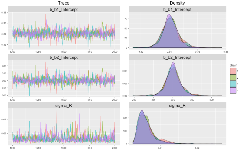
where the vertical lines indicate the values I eyeballed from the wikipedia graph. The model takes a bit of time to compile, but runs four chains rapidly, and the results from the summary are:
Family: gaussian (identity)
Formula: R ~ b1 * S/(b2 + S)
Data: mmk (Number of observations: 9)
Samples: 4 chains, each with iter = 2000; warmup = 1000; thin = 1;
total post-warmup samples = 4000
WAIC: Not computed

Fixed Effects:
   Estimate Est.Error l-95% CI u-95% CI Eff.Sample Rhat
b1_Intercept     0.34      0.01     0.33     0.35       1037    1
b2_Intercept   301.21     20.27   263.30   343.05       1084    1

Family Specific Parameters:
   Estimate Est.Error l-95% CI u-95% CI Eff.Sample Rhat
sigma(R)     0.01         0        0     0.01        835 1.01
And the results for 

Rhat. We can plot our results with the new (in brms 0.8) marginal_effects function, and also plot the MCMC chains with plot (fit2). (The latter graph is included at the top of this posting.)
plot (marginal_effects (fit2), ask = FALSE)

plot (fit2)
The trace plot is a bit clumpier than trace plots we’ve looked at before, but then again we only have 8 data points. There are many details about non-linear regression that I don’t know much about — biases of sigma, perhaps, and others — so this isn’t a tutorial, but hopefully it points you in the right direction if non-linear regression is a path you want to tread.
Bayesian modeling is flexible because it’s really a generalized mechanism for probabilistic inference, so we can create almost any model you can imagine in a flexible tool like Stan. And now brms provides easy access to a very different kind of model than most of us are used to.

Thanks for the interesting post! :-)
As you say, one has to be careful with non-linear models, among others because it’s easy to specify models that are not uniquely identified. That’s why brms requires priors on non-linear parameters, but even then model identification might be problematic sometimes, especially when priors are wide. Of course, frequentist methods have the same problems with identifiability, but without the possibility of setting priors they may be even more complicated to solve.
In addition, Bayesian MCMC methods allow to naturally compute predicted values including credible intervals, without using normal approximations or bootstrapping, as can be seen in the marginal-effects plot.