This is a quick introduction to using R, the R package `knitr`, and the markdown language to automatically generate monthly reports.

Let’s say I track electricity usage and expenses for a client. I initially spent a lot of time analyzing and making models for the data, but at this point I’m now in more of a maintenance mode and simply want an updated report to email each month. So, when their new electricity bill arrives I scrape the data into R, save the data in an R workspace, and then use knitr to generate a simplistic HTML report.

There are three components to make the report. The first is a language called markdown. It’s meant as a simple language for writing basic text that will be turned into basic formatted HTML. It’s designed to look a lot like what people historically used in emails and online postings before HTML was widely used for that purpose. For example, to make a word italic, you would put asterisks around it *like this*. To make a title, you would type your title, then on the next line you’d “underscore” it with hyphens. To make a bullet list, you’d begin each line with an asterisk. And so on. You run the markdown file through a translator, and out comes HTML.

The second component is the `knitr` R package. It enhances markdown to include the ability to execute R code and to substitute the code, the results of the code, or both, into the output HTML. Inline R is placed within back ticks, like `r sum (1:5)`, while more extensive R code is placed in lines bracketed by triple back ticks, where the first line has “{r ” (no quotes) followed by a chunk name, a comma, and options:

```{r part2, echo=T}

So I could write a simplistic report like:

```{r setup, echo=F}
setwd ("~/Documents/Customer/Utilities")
load ("Customer Utilities.Rdata")
opts_chunk$set (
echo=F,
dev="png",
fig.path="figure/",
fig.keep="high",
fig.align="center",
fig.show="hold",
fig.align="center",
comment=NA) 
```

Monthly Electricity Report for `r format (Sys.Date (), "%B %d %Y")`
=======================================================
# Summary

```{r predict, echo=F}
l1 <- lm (daily ~ temp/I(dca-55) - 1, data=elect5)
pred <- sum (predict (l1, n.ahead=6, newdata=data.frame (dca=rep (70, 6), temp=factor (rep ("warmer", 6)))))
last_six <- sum (tail (x2$Total.Current.Charges, 6))
usage.normal <- T
```

Electricity usage last month was `r format (tail (elect5$usage, 1), big.mark=",")` kWh, and expenses were \$`r format (tail (x2$Total.Current.Charges, 1), big.mark=",")`. Last six months usage is `r last_six`, which `r ifelse (usage.normal, "is within", "exceeds")` our normal usage. Projected usage for the next six months is `r pred`.

```{r Plot1, fig.width=7, fig.height=6}
plot (elect5$date, elect5$dollars, main="Electricity Usage", ylab="Daily Average kWh", xlab="Date", type="l")
```

# Techie Details
The formula used for the projected usage is `r format (formula (l1))`, and the $R^2$ is `r summary (l1)$adj.r.squared`.

```{r summary, echo=T}
summary (l1)
```

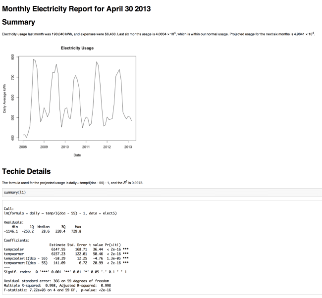
Where the opts_chunk$set is a knitr call to set default options for chunks, such as whether to display the R code (echo). This markdown code would create an HTML report that looks like:

Which is a reasonable start at a report that could be run automatically and emailed or uploaded to a website.

The last component of the trio is the knitr commands that are used within R to process the markdown file (let’s call the markdown file “knitrReport.Rmd”):

library (knitr)
knit2html ("knitrReport.Rmd")
browseURL ("knitrReport.html")

Put the three parts together and you have a dynamically-generated report that can show just the results or can include the R code that was used to generate the results.