An incredible pair of glasses for kids that lets adults adjust them without formal training. It uses two lenses with a liquid between them and a small attachment for adding or removing the liquid to adjust them. (More liquid creates more of a bulge, creating a stronger prescription, less goes the other way.) If it works as well a advertised, it could revolutionize education throughout most of the world.
Stata 13 is nice
I’m a big fan of R, and it will be my primary tool for a long time, but I wanted to add another tool to my toolbox and decided on Stata. Stata 13 was just released (June 2013), and I have to say that it’s a very nice package.
Why would anyone pick Stata over R? R has many advantages, but here are some reasons that you might pick Stata:
Continue reading
Electricity Usage in a High-rise Condo Complex pt 6 (discussion of model)
In Part 4 of this series, I created a Bayesian model in Stan. A member of the Stan team, Bob Carpenter, has been so kind as to send me some comments via email, and has given permission to post them on the blog. This is a great opportunity to get some expert insights! I’ll put his comments as block quotes:
That’s a lot of iterations! Does the data fit the model well?
I hadn’t thought about this. Bob noticed in both the call and the summary results that I’d run Stan for 300,000 iterations, and it’s natural to wonder, “Why so many iterations? Was it having trouble converging? Is something wrong?” The stan command defaults to four chains, each with 2,000 iterations, and one of the strengths of Stan‘s HMC algorithm is that the iterations are a bit slower than other methods but it mixes much faster so you don’t need nearly as many iterations. So 300,000 is a bit excessive. It turns out that if I run for 2,000 iterations, it takes 28 seconds on my laptop and mixes well. Most of the 28 seconds is taken up by compiling the model, since I can get 10,000 iterations in about 40 seconds.
So why 300,000 iterations? For the silly reason that I wanted lots of samples to make the CI’s in my plot as smooth as possible. Stan is pretty fast, so it only took a few minutes, but I hadn’t thought of implication of appearing to need that many iterations to converge.

Electricity Usage in a High-rise Condo Complex pt 5
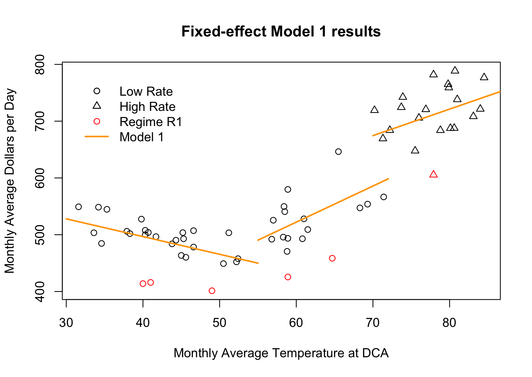
Last time, we modeled the Association’s electricity expenditure using Bayesian Analysis. Besides the fact that MCMC and Bayesian are sexy and resume-worthy, what have we gained by using Stan? MCMC runs more slowly than alternatives, so it had better be superior in other ways, and in this posting, we’ll look at an example of how. I’d recommend pulling the previous posting up in another browser window or tab, and position the “Inference for Stan model” table so that you can quickly consult it in the following discussion.
If you look closely at the numbers, you may notice that the high season (warmer-high, ratetemp 3, beta[3]) appears to have a lower slope than the mid season (warmer-low, ratetemp 2, beta[2]), as was the case in an earlier model. This seems backwards: the high season should cost more per additional kWh, and thus should have a higher slope. This raises two questions: 1) is the apparent slope difference real, and 2) if it is real, is there some real-world basis for this counter-intuitive result?
Continue reading
New R-related website
There’s a new R-related website out there: Rdocumentation, which gathers the documentation for most R packages (that are hosted on CRAN) in one place and allows you to search through it.
There are a couple major benefits to the site:
- It also provides a comments area where you can share thoughts, questions, and tips on various packages or even individual functions. (Though we’ll have to see if a critical mass builds for this.)
- If you search in your own R installation with ?? you will only search the packages you have installed. I’m a package junkie, so have a huge number installed, but it’s still nice to have a place where I can discover new packages more easily.
So check it out and make suggestions to the creators. This should really be rolled into CRAN at some point.
Electricity Usage in a High-rise Condo Complex pt 4
This is the fourth article in the series, where the techiness builds to a crescendo. If this is too statistical/programming geeky for you, the next posting will return to a more investigative and analytical flavor. Last time, we looked at a fixed-effects model:
m.fe <- lm (dollars ~ 1 + regime + ratetemp * I(dca - 55))
which looks like a plausible model and whose parameters are all statistically significant. A question that might arise is: why not use a hierarchical (AKA multilevel, mixed-effects) model instead? While we’re at it, why not go full-on Bayesian as well? It just so happens that there is a great new tool called Stan which fits the bill and which also has an rstan package for R.
Models, Statistical Significance, Actual Significance
“Sometimes people think that if a coefficient estimate is not significant, then it should be excluded from the model. We disagree. It is fine to have nonsignificant coefficients in a model, as long as they make sense.” Gelman & Hill 2007, page 42
“Include all variables that, for substantive reasons, might be expected to be important.” Ibid, page 69.
When a field adopts a common word and uses it in a technical sense, it’s sometimes lucky and sometimes unlucky.
Continue reading
Creative Data Visualization
One of my favorite geographic visualizations is by Neil Freeman, where he took a map of the U.S. and kept the physical boundaries and cities, but morphed state boundaries (and renamed them as well) to create a map with 50 states, each with equal population. It’s a pretty amazing mixture of real maps, real data, and imagination.

Electricity Usage in a High-rise Condo Complex pt 3
In a previous installment, we looked at modeling electricity usage for the infrastructure and common areas of a condo association, and a fairly simple model was reasonably accurate. This makes sense in a large system such as mid-sized, high-rise condo building, which has a lot of electricity-usage inertia. The cost of that electricity has a lot more variability, however, because of rate changes (increases and decreases), refunds, high/low seasons, and other factors that affect the bottom line.
Customer Service: Three Strikes in One Day
I’ve been using R for years, but decided that I should broaden my horizons (and resumé), so I decided to sign up for an SAS class at the local university, my graduate alma mater. It’s been a couple of hours since that decision and I’ve gotten three vivid lessons in what Customer Service is not. Continue reading
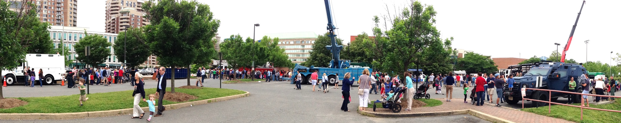
Truck Day in Arlington
On a less-technical note (and we will get back to electricity), the Arlington County Public Library held their annual Truck Day today. Here’s a panoramic shot that shows many but not all of the trucks. The fire truck was there for a while, but had to leave for a fire. The police swat truck is on the far right, and beyond it you can see the bus. I wouldn’t have expected it, but the longest lines were to get on the bus!
Electricity Usage in a High-rise Condo Complex pt 2
In a previous installment, we described a condo association that needed to know what its electricity budget should be for an upcoming budget. In this posting, we’ll develop a model for electricity utilization, leaving electricity expenses for the next installment.
I like to have pretty pictures above the fold, so let’s take a look at the data and the resulting model, all in one convenient and colorful graph. The graph shows each month’s average daily electricity usage (in kilowatt hours, kWh) versus the month’s average temperature at nearby Ronald Reagan Airport (DCA). Each month’s bill is a point at the center of the month name:

Electricity Usage in a High-rise Condo Complex pt 1
This is the story of a condominium association in Northern Virginia, which was in the midst of transforming their budget. In the early days of the association they didn’t have an operational cash reserve built up, so they had to make budget categories a bit oversized, “just in case”. As time went on, they saved the cash from their over-estimates, and eventually arrived at the place where they could set tighter budgets and depend on their cash savings if the budget were exceeded.
In the process of reviewing various categories, they came to “Utilities”, which lumped water, sewage, gas, and electricity all together. They decided to break it down into individual utilities, but when they started with electricity, no one actually knew how much was used nor how much it cost. The General Manager had dutifully filed away monthly bills from Dominion, but didn’t have a spreadsheet. They needed a data analyst, and I was all over it.
In the next four or five postings, I want to show some of the details of my investigation of electricity expenses. I hope it will be an interesting look at the kinds of things that happen in the real world, not just textbooks. Oh, by the way, it turns out that electricity was the single largest operating expense of the association. Here’s a graph of average expenditures, brought up to the present:

Lots of Free Data is Good
Francis Smart, over at the Econometrics by Simulation blog has a great introduction to the Quandl website. Quandl has a boatload of searchable financial, economic and social datasets, and one can never have too much data.
And Vincent Granville, over at Big Data News has a post about Enigma which also has lots of data links.
What a good time to be into Data Analytics!
R’s reshape Function
The reshape function in R is very useful, but poorly documented. Wingfeet, over at Wiekvoet, has written a well-illustrated article on reshape that steps through SAS’ transpose examples and shows how that’s done with R’s reshape.
Automatic Report Generation in R, with knitr and markdown
This is a quick introduction to using R, the R package `knitr`, and the markdown language to automatically generate monthly reports.
Let’s say I track electricity usage and expenses for a client. I initially spent a lot of time analyzing and making models for the data, but at this point I’m now in more of a maintenance mode and simply want an updated report to email each month. So, when their new electricity bill arrives I scrape the data into R, save the data in an R workspace, and then use knitr to generate a simplistic HTML report.
14,000-year-old Words and Wordplay
Language fascinates me, though I took German in High School and never did well, and I’m currently struggling to learn Spanish (though I learn computer languages easily). So while I struggle with particular (human) languages, language itself absolutely fascinates me. Years ago, I also took ancient Greek for three semesters and remember my professor wondering aloud whether the Greek language is flexible because Greeks were philosophers, or whether Greeks became philosophers because their language was so well-adapted to discussing abstract concepts.
Two language-related items today:
First, I highly recommend the book Word Play, by Peter Farb. It talks about everything from how many names for colors languages have and African word competitions, to euphemisms and honorific languages.
Second, the PNAS has an article, “Ultraconserved words point to deep language ancestry across Eurasia” looking at words that have been preserved in various ways for perhaps as long as 14,500 years. The PDF is not paywalled, so you can download it if you want. The abstract is:
Creative and Inspiring Architecture
When I was in Junior High School, I wanted to be an architect. I even took a drafting class, and in my spare time designed a city. Never got around to designing actual buildings before my interests turned to physics, then photography, and finally computers.
I still find good architecture to be amazingly inspiring. There’s something about architecture that makes it special: it’s like a monument or a sculpture, but it’s also a space that is itself planted in a space and has a flow. I’ve tweeted about interesting buildings a few times and highly recommend Wired Magazine’s Building-of-the-week page.
Here’s a local building that does three things at once: 1) it has an interesting and attractive design, 2) it has several parts that join the building with a couple of different surrounding architectures, and 3) it includes a replica of the previous building as an element in its design. So it spans both space and time. Very classic.

A Brief Tour of Tree Packages in R
A Brief Tour of Tree Packages in R
Good news about R is it has thousands of packages. Bad news about R is that it has thousands of packages, and often it’s difficult to know which wavelet packages, for example, do what.
On his blog, Wes has provided a concise, illustrated tour of the major tree/forest packages in R. Go and gain clarity.
It’s the Little Differences That Matter
Everyone’s interested in the global climate these days, so I’ve been looking at the GISTEMP temperature series, from the GISS (NASA’s Goddard Institute for Space Studies). I was recently analyzing the data and it turned into an interesting data forensics operation that I hope will inspire you to dig a little deeper into your data.
Let’s start with the data. GISS has a huge selection of data for the discerning data connoisseur, so which to choose? The global average seems too coarse — the northern and southern hemispheres are out of phase and dominated by different geography. On the other hand, the gridded data is huge and requires all kinds of spatially-saavy processing to be useful. (We may go there in a future post, but not today.) So let’s start with the two hemisphere monthly average datasets, which I’ll refer to as GISTEMP NH and GISTEMP SH.
To be specific, these time series are GISTEMP LOTI (Land Ocean Temperature Index) which means that they cover both land and sea. GISS has land-only data and combines this with NOAA’s sea-only data from ERSST (Extended Reconstructed Sea Surface Temperature). I’d also point out that all of the temperature data I’ll use is measured as an anomaly from the average temperature over the years 1951-1980, which was approximately 14 degrees Celsius (approximately 57 degrees Farenheit). So let’s plot the GISTEMP LOTI NH and SH data and see what we have.

Bayesian Data Analysis 3
In the first posting of this series, I simply applied Bayes Rule repeatedly: Posterior 


Well, first, there’s really no good way for me to communicate my
Second, my posterior density is discrete. This works reasonably well for the exercise I attempted, but it’s still a discrete approximation which is less precise and can suffer from simulation-related issues (number of samples, etc) that have nothing to do with my proposed model.
Third, if an analytical method can be used, it may be possible to directly calculate a final posterior without repeated applications of Bayes Rule. As I mentioned in the previous posting, Gelman got an answer of Gamma(238, 10) analytically, not through approximations and simulation. If we look in Wikipedia, we can find that the conjugate prior for 


Bayesian Data Analysis 2
In the last post (Bayesian Data Analysis 1), I ran a Bayesian data analysis using a simple, first-principles approach. Armed with only the fact that a Poisson distribution is appropriate for modeling airplane accidents, Bayes Rule, and R, we got the correct answer to the problem through non-parametric simulation.
Before we get into precision and the other topics in the list of issues to explore, let’s tie up one loose end. I could have gotten the right answer for the wrong reason, so let’s look at the posterior distribution of 

rgam <- rgamma (20000, 238, 10)
And then we can compare our posterior distribution with the official, parametric distribution:

Looks reasonably close (though biased by about 0.25) and it didn’t take a lot of fancy machinery to pull off. So why not use this method as our default? Why talk of things like conjugate priors and hyper parameters? And did we just get lucky with numeric precision because we only had 10 accidents and hence only 10 applications of Bayes Rule? Let’s cover that in the next posting, and finish this one with a graph of our answer (not

Bayesian Data Analysis 1
I’ve read quite a few presentations on Bayesian data analysis, but I always seem to fall into the crack between the first, one-step problem (the usual being how likely you are to have a disease), and more advanced problems that involve conjugate priors and quite a few other concepts. So, when I was recently reading Bayesian Data Analysis[1], I decided to tackle Exercise 13 from Chapter 2 using only Bayes rule updates and simulation. I think it’s been illuminating, so decided to write it up here, using my favorite tool R.
Exercise 13 involves annual airline accidents from 1976 to 1985, modeled as a Poisson
accidents <- c(24, 25, 31, 31, 22, 21, 26, 20, 16, 22)
A little playing around with graphs and R‘s dpois gives me the impression that
r <- seq (10, 45, 0.2)

theta1 <- dnorm (r, 15, 5)

theta1 <- theta1 / sum (theta1)

theta2 <- dnorm (r, 35, 6)

theta2 <- theta2 / sum (theta2)

theta3 <- 20 - abs (r - mean (r))

theta3 <- theta3 / sum (theta3)
Where theta1 is probably low, theta2 is probably high, and theta3 is not even parametric. (More on this later.) I normalized them to create proper priors so that they graph well together, but that wasn’t necessary. Remember, I’m doing all of my calculations over the discretized range, 

So let’s run the numbers (accidents) through a repeated set of Bayes Rule updates to get a posterior distribution for
600 Years Ago, the Sea Was Space

Looking out at the ocean recently, I got to thinking about the ocean. Living by the ocean. Being tied to the ocean. Being a tiny speck, far out to sea.
And it struck me that 600 years ago, the ocean might have been a lot like outer space is for us. An unforgiving place of danger (still is, in many ways). The unknown, where the era’s high-tech was deployed. A place where your eyes might see what no other eyes had ever seen in all of history. And a place where you and your nation might gain glory.
The high-technology ranged from ship and sail designs to maps, weapons, navigational tools, and even knowing where land was based on clouds forming or making sense of waves reflected and refracted by islands.
In other places and eras, spices were high-tech — flavor-enhancement and health-enhancement in one package — and empires were built on their trade. Roman soldiers’ gear and tactics were high-tech, as were their empire’s roads and other civil engineering projects. At one point, the C&O Canal near where I live was high-tech, obsoleted within a decade or so of its peak by the railroad.
I’ve even read that tea was high-tech in England ~200 years ago: laborers drank ale to soothe weary bodies, information-workers drank tea to boost mental capabilities. (IT industry and caffeine, anyone?)
Now, here I sit, typing on an iPad, wirelessly loading the words via 3G to a server thousands of miles away. I have a Master’s degree in Artificial Intelligence… Or am I a master cartographer who lives by the sea? Guess I’ll just have to listen to the rain falling and the waves crashing to be sure.
